CUDA Programming (5): Program Timing and Performance Metrics

Note: This article is an English translation and adaptation of the original post published on SeanWangJS.github.io.

In high-performance computing, execution time and hardware utilization are the primary measures of software quality. CUDA provides specialized runtime APIs to capture kernel execution intervals on the Device with microsecond precision. In this article, we explore how to measure kernel execution time using CUDA Events, define essential performance metrics (effective memory throughput, compute throughput, and arithmetic intensity), and evaluate performance bottlenecks using the Roofline Model.

1. Kernel Timing with CUDA Events

While standard CPU timers (such as std::chrono) can measure end-to-end execution, they include CPU-GPU synchronization overhead and driver launch latency. To accurately isolate the execution time of a kernel on the Device, CUDA provides CUDA Events [1].

The following code illustrates how to profile a kernel using CUDA Events:

void vectorAdd(const float *a,
               const float *b,
               const int n,
               float *c) {
    
    float *d_a, *d_b, *d_c;
    cudaMalloc((void**)&d_a, n * sizeof(float));
    cudaMalloc((void**)&d_b, n * sizeof(float));
    cudaMalloc((void**)&d_c, n * sizeof(float));

    cudaMemcpy(d_a, a, n * sizeof(float), cudaMemcpyHostToDevice);
    cudaMemcpy(d_b, b, n * sizeof(float), cudaMemcpyHostToDevice);

    int block_size = BLOCK_SIZE;
    int grid_size = (n + block_size - 1) / block_size;

    // Declare start and stop events
    cudaEvent_t start, stop;
    cudaEventCreate(&start);
    cudaEventCreate(&stop);

    // Record start event into the default stream
    cudaEventRecord(start);

    // Launch kernel
    vector_add_kernel<<<grid_size, block_size>>>(d_a, d_b, n, d_c);

    // Record stop event
    cudaEventRecord(stop);

    // Wait until the stop event has been recorded by the GPU
    cudaEventSynchronize(stop);

    // Compute elapsed time in milliseconds
    float time = 0.0f;
    cudaEventElapsedTime(&time, start, stop);
    printf("Kernel Execution Time: %f ms\n", time);

    cudaMemcpy(c, d_c, n * sizeof(float), cudaMemcpyDeviceToHost);

    // Destroy events to free runtime resources
    cudaEventDestroy(start);
    cudaEventDestroy(stop);

    cudaFree(d_a);
    cudaFree(d_b);
    cudaFree(d_c);
}

Key Timing Mechanics

1. Event Creation and Recording: Events are created via cudaEventCreate and queued into the execution stream using cudaEventRecord. Because kernel launches are asynchronous, cudaEventRecord(start) and cudaEventRecord(stop) bracket the kernel in the stream.
2. Event Synchronization: cudaEventSynchronize(stop) blocks the Host thread until the stop event is reached and executed by the GPU, ensuring that all intervening kernel operations have completed.
3. Resolution: cudaEventElapsedTime calculates the time between two recorded events in milliseconds (ms), offering a sub-microsecond resolution (~0.5 µs) independent of CPU clock jitter.

2. Memory Throughput

Once execution time is measured, we can calculate Effective Memory Throughput to assess how efficiently a kernel utilizes memory bandwidth:

Where $N$ represents the total number of bytes read and written during execution, and $t$ is the kernel execution time in seconds. Throughput is typically expressed in GB/s.

For example, in vector addition with $n = 2^{25}$ ($33{,}554{,}432$) elements:

• Each single-precision float occupies $4\text{ bytes}$.
• Each element requires 2 reads ($a[i], b[i]$) and 1 write ($c[i]$), totaling 3 memory transfers.
• Total data moved: $N = 2^{25} \times 4 \times 3\text{ bytes} \approx 0.4027\text{ GB}$ (or $0.375\text{ GiB}$).

If the kernel executes in $t = 2\text{ ms}$ ($0.002\text{ s}$), the effective throughput is:

Comparing this value against the GPU’s theoretical peak bandwidth (e.g., $1555\text{ GB/s}$ on an NVIDIA A100) quantifies the memory bus efficiency of the implementation.

3. Compute Throughput

Complementing memory throughput, Compute Throughput measures the rate of floating-point operations executed per second, expressed in FLOPS (or GFLOPS / TFLOPS):

By comparing achieved compute throughput against the theoretical peak compute performance derived in Part 1 ($19.5\text{ TFLOPS}$ for A100 FP32), we determine how effectively the streaming multiprocessors (CUDA Cores) are kept occupied.

4. Arithmetic Intensity

Arithmetic Intensity (AI) is an intrinsic characteristic of an algorithm, defined as the ratio of floating-point operations performed to bytes of data accessed from global memory:

Algorithms with high arithmetic intensity are computationally dense, while algorithms with low arithmetic intensity spend most of their time transferring data across the memory bus.

Example: Matrix Multiplication ($n \times n$)

Consider a square matrix multiplication $C = A \times B$:

• Each element in $C$ requires a dot product between a row of $A$ and a column of $B$, involving $n$ multiplications and $n-1$ additions ($2n - 1 \approx 2n\text{ operations}$).
• For an $n \times n$ matrix, the total floating-point workload is $n^2 \times 2n = 2n^3\text{ FLOPs}$.
• In the optimal memory scenario (where each element of $A, B$ is fetched once from global memory and $C$ is written once), the minimum data transfer is $3 \times n^2 \times 4\text{ bytes} = 12n^2\text{ bytes}$.

The theoretical upper bound for the arithmetic intensity of matrix multiplication is therefore:

As matrix dimension $n$ scales up, arithmetic intensity increases linearly, transitioning the operation from memory-bound to compute-bound.

5. The Roofline Model

The Roofline Model [2][3] provides an intuitive visual framework for evaluating whether an application is constrained by memory bandwidth (memory-bound) or compute capacity (compute-bound) on a target hardware platform.

Mathematically, attainable performance is governed by two ceiling limits:

Where:

• $P_{\text{peak}}$ is the theoretical peak compute throughput (e.g., $19{,}500\text{ GFLOPS}$ on A100 FP32).
• $\text{BW}_{\text{peak}}$ is the theoretical peak memory bandwidth (e.g., $1555\text{ GB/s}$ on A100).
• $\text{AI}$ is the arithmetic intensity of the workload.

The turning point (or “knee” of the roofline) occurs at:

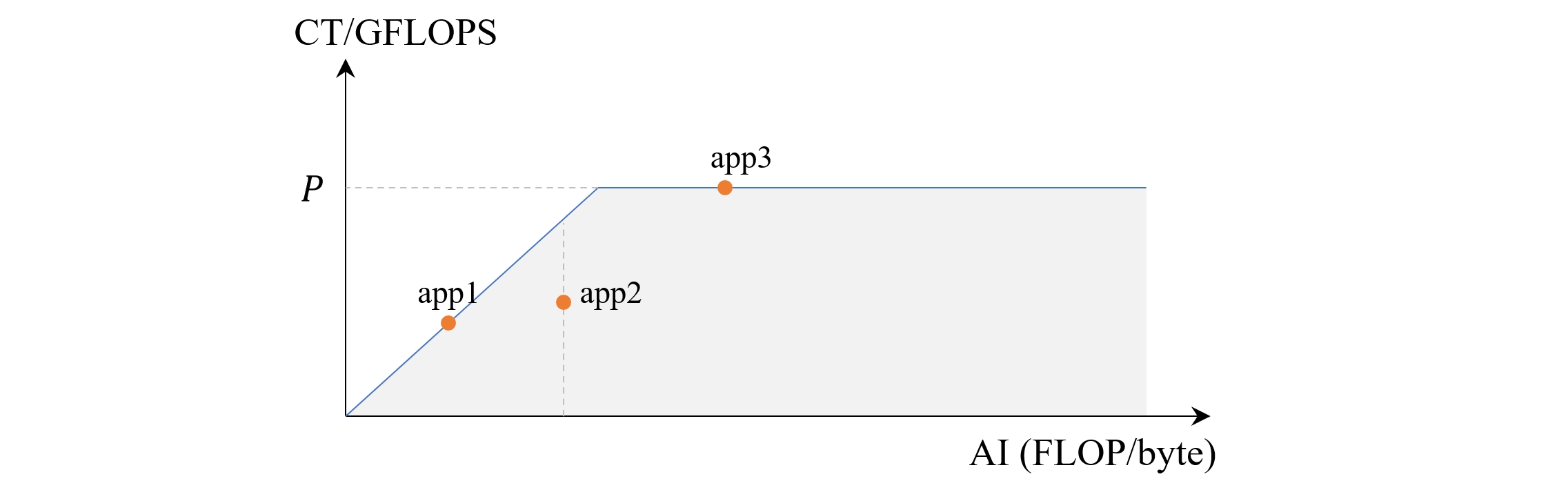Figure 5.1: The Roofline Model [3]

Interpreting the Model

• Slanted Region ($\text{AI} < \text{AI}_{\text{knee}}$): The workload is memory-bound. Compute units sit idle waiting for operands from memory. Optimization efforts must focus on improving memory access patterns, coalescing, and caching in Shared Memory or registers.
• Flat Region ($\text{AI} > \text{AI}_{\text{knee}}$): The workload is compute-bound. Memory bandwidth is sufficient, but raw arithmetic throughput is saturated. Optimization efforts must focus on instruction-level parallelism, loop unrolling, or moving to Tensor Cores.
• In Figure 5.1:
  • App 1: Hits the memory ceiling. To improve throughput, its arithmetic intensity must be increased, or redundant memory transfers eliminated.
  • App 2: Sits below the memory roofline; its memory access pattern is inefficient, meaning performance can be boosted by improving memory coalescing and cache locality.
  • App 3: Operates in the compute-bound regime at peak hardware capacity.

References

• NVIDIA Corporation, How to Implement Performance Metrics in CUDA C/C++, NVIDIA Technical Blog.
• Zhihu, Roofline Model and Deep Learning Performance Analysis.
• Wikipedia, Roofline Model.